Real-time visualization with Rerun
easy
visualizaztion
operations
plugin
Abstract
Rerun.io is a powerful tool for real-time visualization and debugging of robotics applications. This guide introduces the rerunner plugin, which allows to capture MADS packets and feed them to the rerun viewer to get real-time plots of signals.
Introduction
Rerun.io is a powerful tool for real-time visualization and debugging of robotics applications. It allows developers to visualize data from their applications in real-time, making it easier to identify issues and understand system behavior. It supports visualization of 2-D plots and time-series, 3-D cloud points and scenes, tabulated data, heatmaps and tensor maps. Rerun is made by two components: The library, which is integrated into the application to capture and send data, and the viewer GUI, which displays the data in a user-friendly interface.
The rerunner plugin is a MADS sink plugin that integrates the Rerun library into MADS. It captures MADS packets and feeds them to the Rerun viewer, allowing users to visualize data from their MADS applications in real-time.
The plugin
Installation
To obtain and install the plugin, follow instructions on the GitHub page. Note that you’ll have to download separately the Rerun library, as described in the instructions or following this link. Once you have compiled and installed the plugin, you can quickly test it together with the replay source plugin, which is used to publish a previously recorded MADS log file. In the following, we are assuming that you have it installed and that followed its guide.
Usage
Keypaths
The plugin uses the concept of keypaths to tap into JSON messages and extract data to be sent to the Rerun viewer. A keypath is a string that specifies the path to a specific field in a JSON object, using slash notation to separate nested fields. For example, the keypath /sensor/temperature would refer to the temperature field inside the sensor object:
{
  "sensor": {
    "temperature": 25.3,
    "humidity": 60
  }
}
Furthermore, the plugin can subscribe to multiple MADS topics, so a keypath is actually prepended with the topic name. So, according to the example above, if the message is published on the topic env, the full keypath to access the temperature field would be /env/sensor/temperature.
If a JSON object contains an array, you can use numbers to access individual elements. For example, the keypath /sensors/0/temperature would refer to the temperature field of the first element in the sensors array:
{
  "sensors": [
    {
      "temperature": 25.3,
      "humidity": 60
    },
    {
      "temperature": 26.1,
      "humidity": 55
    }
  ]
}
Important
Keypaths must start with a leading slash: /sensor/x os OK, sensor/x is wrong.
An alternative syntax uses dots and square brakets for array indexes, as for example in topic.sensor[0].temperature. This alterante syntax less efficient and it is mostly supported for similarity to the replay plugin.
Visualizations
The plugin supports the visualization of scalar values as time series. If the INI file contains the following section:
[rerunner]
sub_topics = ["env"]
keypaths = ["/env/sensor/temperature", "/env/sensor/humidity"]
then the Rerun viewer will display two time series for the temperature and humidity values. The layout of the two series is heuristically determined by the viewer, but it can be customized by the user in the viewer GUI.
The INI file can also contain an array of trace keypaths. a trace is a sequence of 2-D or 3-D points that can be used to visualize trajectories, paths, or any other sequence of points. For example, if the JSON messages contain a field position with the following structure:
{
  "position": [1, 2, 3]
}
then the keypath to visualize the position as a trace would be trace_keypath = ["/env/position"]. The plugin will automatically detect that this is a 3-D point and will visualize it as such in the Rerun viewer. If the position field contains only two values, it will be visualized as a 2-D point.
For the time-series, the plugin assumes that the JSON messages contain a field named timeframe with the timeframe of the measurement, expressed in seconds since last midnight rounded to the nearest frame. If the field is not present, the plugin will use the current system time as timestamp.
At the moment, the plugin can also visualize the Auto-Correlation Function (ACF) and Fast Fourier Transform (FFT) of selected signals. The ACF is useful for visualizing periodicity in the signal and — most importantly — to define the maximum sampling frequency for a signal (above that frequency we are essentially sampling the same observation).
To also plot ACFs and FFTs, select the desired signals and set the running window size as follows:
window_size = 500
acf_keypaths = ["/env/sensor/temperature", "/env/sensor/humidity"]
fft_keypaths = ["/env/sensor/temperature", "/env/sensor/humidity"]
The plugin currently also calculates, for each selected signal, its average, standard deviation, and standard uncertainty. Also, it provides statistics on the time-steps.
TipMore complex viewers
It is relatively easy to customize the RerunnerPlugin class to add more or different viewers, including animating 3-D scenes with real-time data. Follow the Rerun guides for that.
Paths in Rerun
The Rerun viewer receives data organized in paths, using the same slash syntax above described. You can expect the followings:
data/*: the raw data as time seriesacf_plot/*: the autocorrelation function plotsfft_plot/*: the autocorrelation function plotsstats/mean/*: the running mean for the same signals indata/stats/stdev/*: the running standard deviation for the same signals indata/stats/std_uncertainty/*: the running standard uncertainty for the same signals indata/timestep: the time series of data timestepsmean_timestep: the running mean for the data timesteps
Using the Rerun viewer GUI it is easy to add/remove and rearrange plots for individual data series.
Rerun blueprints
The Rerun viewer supports blueprints. A blueprint is actually a description of the panels layout in the viewer and of their content (type and configuration of graphical elements). In the absence of a blueprint specified by the user, the Rerun viewer heuristically creates one by itself. Starting from that, the user can rearrange panels and charts to his/her likings, and then save the blueprint as a .rbl file.
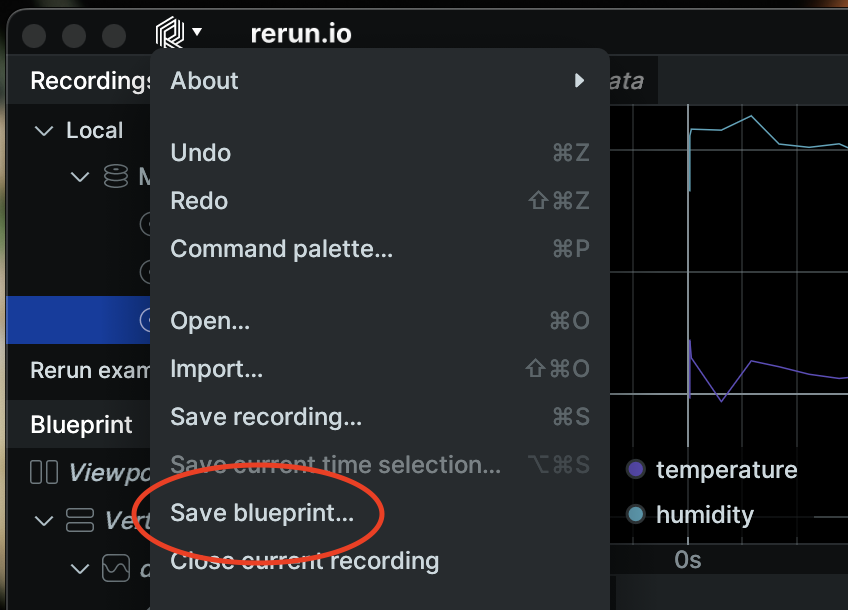
Once you have a blueprint file, you can load it upon launching the rerunner.plugin, in two different ways:
- by adding a line
blueprint = "path/to/a/.rbl/file"to the[rerunner]INI section - by passing the option to the plugin command line:
mads sink rerunner.plugin -o blueprint=path(this requires mads version 1.4.x)
The command line options overrides any settings in the INI file.
Example usage
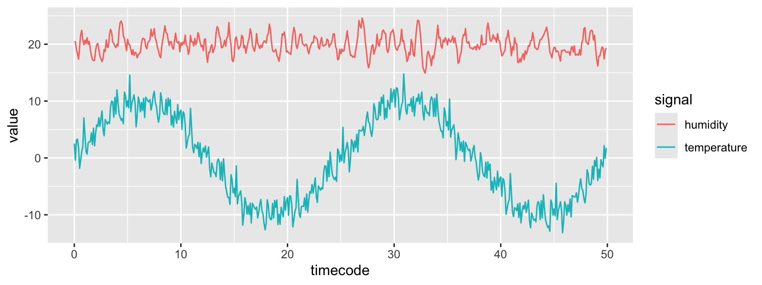
We are using the replay plugin to reproduce in loop a CSV file generated with synthetic data. The datafile contains two signals, sensor.temperature and sensor.humidity, published on the topic replay. The temperature signal is generated with a sinusoidal plus some Gaussian noise. the humidity signal is generated with as an ARIMA(2,0,4) process, so that we expect to have 3-4 lags of autocorrelation.
The ACF and PACF charts of the humidity signal are:
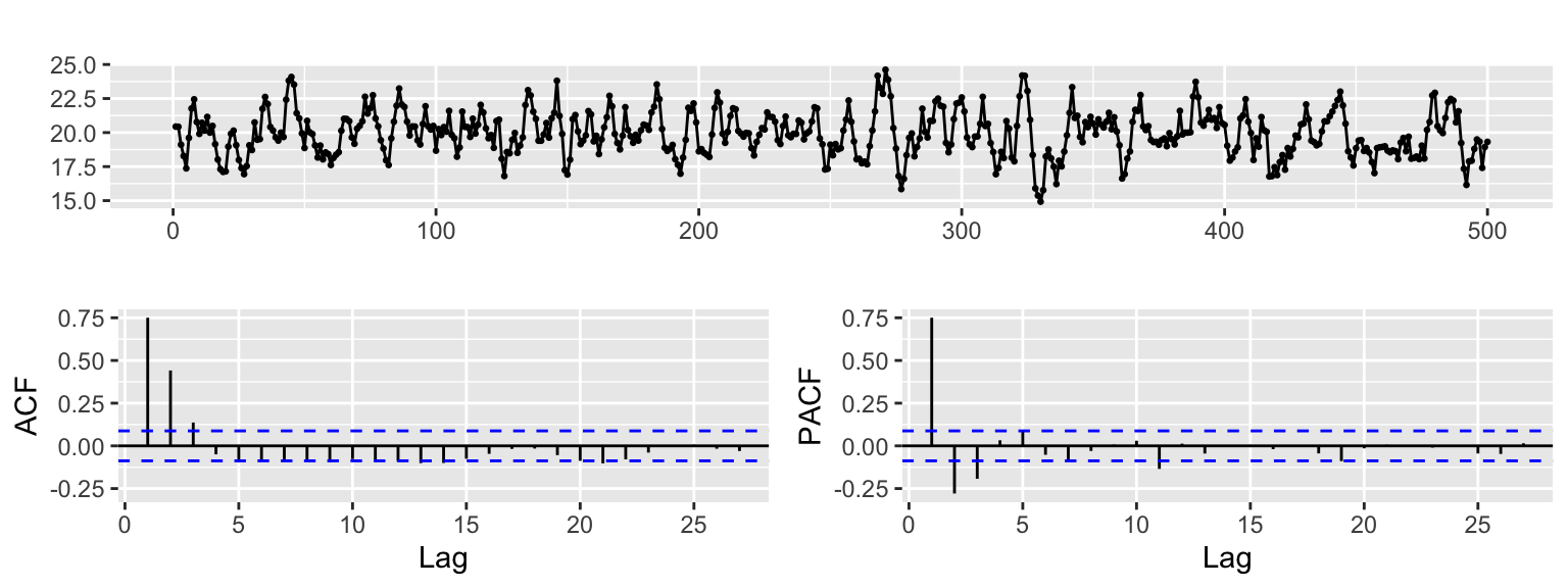
We observe that in the ACF chart the lags 1–3 are significant.
These data are available in the example.csv file in the rerunner_plugin repository.
To quickly test the rerunner plugin, we follow the next steps:
- Install the
replaysource plugin - Start the MADS broker
- Configure the
replay.pluginwith this INI section:
[replay]
pub_topic = "replay"
period = 10
csv_file = "example.csv"
loop = true- Clone the
rerunnerplugin:git clone https://github.com/MADS-NET/rerunner_plugin.git - From the
rerunner_pluginfolder, run thereplayplugin, so that it uses theexample.csvfile from the current folder:
mads source replay.plugin- Configure the INI file withe the following:
[rerunnner]
sub_topic = ["replay"] # Topics to subscribe
time = ""              # Use system time
window_size = 200      # ACF running windows width
keypaths = ["/replay/sensor/temperature", "/replay/sensor/humidity"]
acf_keypaths = ["/replay/sensor/temperature", "/replay/sensor/humidity"]
fft_keypaths = ["/replay/sensor/temperature", "/replay/sensor/humidity"]- Launch the Rerun viewer
- From a new terminal, compile and launch the
rerunnerplugin:
cmake -Bbuild -DCMAKE_INSTALL_PREFIX=$(mads -p)
cmake --build build -j6
mads sink build/rerunner.plugin- The plugin will start collecting the data streamed on the
replaytopic and plotting it on the viewer:
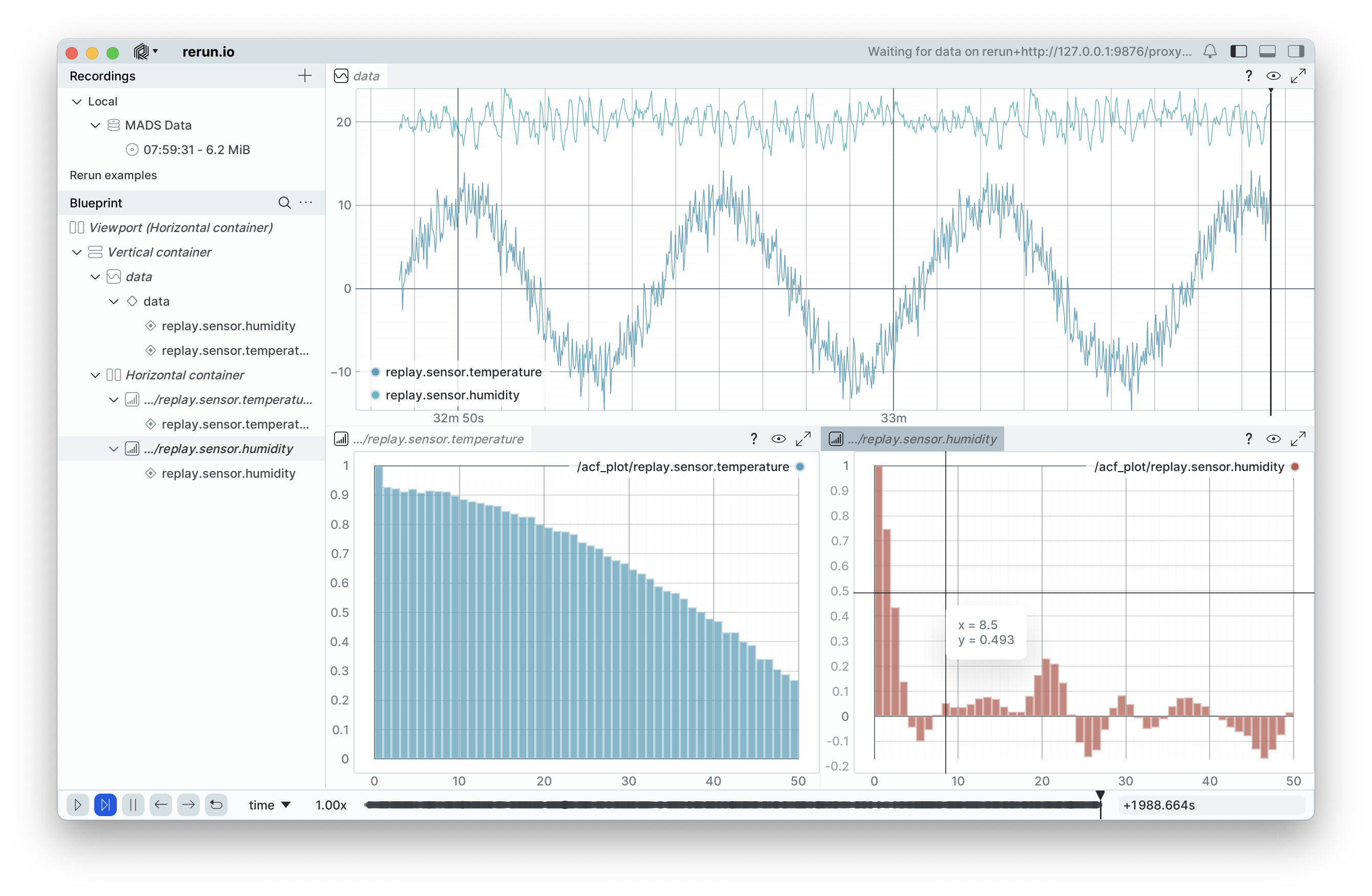
In particular, note that the ACF file for the humidity signal shows significant lags at 1, 2 and 3, as expected, while the temperature signal a long ACF as expected by such a periodic signal.